Tutorial
How to import the library
beanPy can be imported by putting beanPy in your workspace and running
>>> import beanPy as Beans
For all of the guides it is implied that you have aready imported the library into your workspace
How to define a distribution
beanPy has an assortment of different distributions to use such as
Normal
This defines a normal distribution given a defined mean_value and variance_value
our_normal_distribution = Beans.NormalDistribution(mean_value, variance_value)
Exponential
This defines an exponential distribution given a defined lambda_value
our_exponential_distribution = Beans.ExponentialDistribution(lambda_value)
Poisson
This defines an poisson distribution given a defined lambda_value
our_poisson_distribution = Beans.PoissonDistribution(lambda_value)
Continuous uniform
This defines a continous uniform distribution given a defined min_value, max_value
our_continous_uniform_distribution = Beans.ContinuousUniformDistribution(min_value, max_value)
Discrete uniform
This defines a discrete uniform distribution given a defined min_value, max_value and an optional step_value
our_discrete_uniform_distribution = Beans.DiscreteUniformDistribution(min_value, max_value, [step_value])
Note: The default value of step_value is 1, so if omitted it will default to step_value = 1
The min_value is always included in the distribution however if you give a max_value and the step_value cannot step towards it it will reduce the max_value such that the largest number of steps are included
For example:
>>> mean_value = 0
>>> variance_value = 1
>>> our_normal_distribution = Beans.NormalDistribution(mean_value, variance_value)
This will define a standardized normal distribution, of course you could always parse the mean and variance directly into our function
How to take samples with a chosen distribution
The main use of our library is to take samples of numbers with a given distribution. To do so you must define a distribution and define number_of_samples and seed then parse
our_chosen_distribution.TakeSample(seed)
Or in order to take multiple samples at once you parse
our_chosen_distribution.TakeMultipleSamples(number_of_samples, seed)
The seed can be omitted in both of these cases
For example:
First we define the distribution, in this case using standardized normal so that you can check it against other values online.
>>> mean_value = 0
>>> variance_value = 1
>>> our_normal_distribution = Beans.NormalDistribution(mean_value, variance_value)
Now you generate a sample of numbers in preportion to the normal distribution
>>> number_of_samples = 1000
>>> seed = 0
>>> our_normal_distribution.TakeMultipleSamples(number_of_samples, seed)
This will output 1000 samples of numbers in the preportion of the normal distribution
To test if this has given us a suitable output, test the samples mean (\(\mu\)) and variance (\(\sigma^2\))
>>> output = our_normal_distribution.TakeMultipleSamples(number_of_samples, seed)
>>> sample_mean = sum(i for i in output) / number_of_samples
>>> #using the equation of variance
>>> sample_variance = sum(i ** 2 for i in output) / number_of_samples - sample_mean
>>> print(f"μ = {sample_mean}, σ² = {sample_variance}")
Giving us
\[\mu = 0.04904221840834106, \sigma^2 = 0.9342589470547096\]
This has generated a list of numbers with, approximatley, a mean 0 and a variance 1. Obviously with more samples it will be closer to the desired mean and variance since the sample size would be larger
How to find quantiles of a defined distribution
For any of the distributions \(X\) you can find their quantiles, which is to find the value of \(x\) at which the probability of something happening is less than or equal to a probability you parse into it. In other words to find \(x\) given \(p\)
To do this you must define a distribution and parse
probability_value = p
our_chosen_distribution.FindQuantile(probability_value)
For example:
Using the standardized normal distribution so that we can check we get the correct value of the quartile
>>> mean_value = 0
>>> variance_value = 1
>>> our_normal_distribution = Beans.NormalDistribution(mean_value, variance_value)
Now use the FindQuantile function on the our_normal_distribution
>>> our_probability = 0.95
>>> our_normal_distribution.FindQuantile(our_probability)
\[x = 1.16308715367667 \sqrt{2}\]
beanPy uses sympy to compute its functions so it is returned as much of an exact value as it can, obviously when you use this code you may want to just see the decimal value, hence we return the value as a float
>>> float(our_normal_distribution.FindQuantile(our_probability))
\[x = 1.6448536269514724\]
We can see if this is true by looking at a table of standardized normal values you can see that
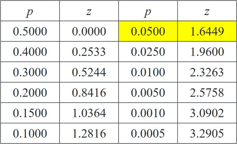
And hence have found the quantile of our defined distribution
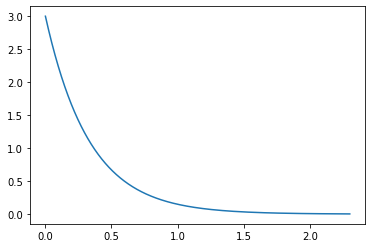
How to plot a PDF of a distribution with given parameters
For all of the supported distributions of beanPy you can plot them on the graph to have a visualization of how the numbers generated are spread, the library supports being able to change the number of points to draw the graph with - in order to get the required level of accuracy with a speed. To do this you must define a distribution and parse.
number_of_points = 100
our_chosen_distribution.PlotPDF(number_of_points)
You can omit number_of_points and it will default to 50 points
For example:
Using the exponential distribution for this example
>>> lambda_value = 3
>>> our_exponential_distribution = Beans.ExponentialDistribution(lambda_value)
For any of the distributions 1000 points is a good balance of speed to accuracy of graph, so we will be using that for ours but it defaults to 50 if nothing given
>>> number_of_points = 1000
>>> our_exponential_distribution.DrawPDF(number_of_points)
And hence have our PDF curve